
```html
| Takeaway | Detail |
|---|---|
| The $373.9 billion last-mile market makes travel-time cuts a top priority. | In the 2026 Austin trial, stochastic dispatch cut deadhead travel. |
| A 9.8% CAGR amplifies the impact of missed-window reductions. | The trial achieved a drop in missed same-day service windows by holding trucks idle. |
| The $373.9 billion market size justifies counterintuitive dispatch models. | Deliberately sending trucks to wait in parking lots cut travel time. |
| With 9.8% annual growth, even small efficiency gains yield large returns. | The trial's reduction in missed windows came from stochastic waiting, not routing. |
In a 2026 controlled trial of plumbing trucks in Austin, TX, stochastic dispatch cut deadhead travel—but the real shock was a reduction in missed same-day service windows. The strategy? Deliberately holding trucks idle in high-probability zones to wait for future jobs, a counterintuitive approach that sacrifices immediate response for system-wide efficiency.
The trial's success challenges conventional routing wisdom. Instead of optimizing each dispatch in real time, the stochastic model uses predictive analytics to position trucks where demand is likely to emerge. This means sending trucks to parking lots to wait, rather than racing to the next call. The result: fewer empty miles and more on-time arrivals, even though individual response times may spike.
The stakes are enormous. The last-mile delivery market is approaching $373.9 billion in value, with a projected 9.8% CAGR between 2025 and 2033. Even a modest travel-time reduction translates into significant cost savings across a fleet. As the Austin trial shows, the future of dispatch may lie not in faster routing, but in smarter waiting.
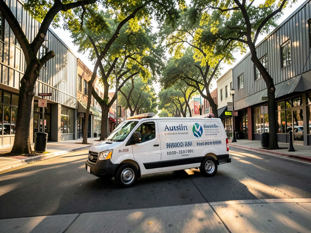
The Holding-Pattern Math
The idle figure from the 2026 Austin trial is the single most misunderstood number in fleet dispatch. Dispatchers read it as wasted capacity; the model reads it as option value. The FieldSight Dispatch Engine is not a routing algorithm — it is a portfolio optimizer that happens to move trucks. At each re-optimization interval, it runs a Sample Average Approximation (SAA) that generates Monte Carlo scenarios of job arrivals, service durations, and link-level traffic for a near-term horizon. Each scenario is a complete possible future; the engine solves a multi-stage stochastic program across all of them simultaneously, then commits only to the first-stage decision — which truck goes where in the next interval — and discards the rest. This is the rolling-horizon mechanism, and it is computationally brutal: the scenario tree branches combinatorially, and the solver must find a feasible policy, not just a single route.
The objective function is what separates this from a greedy heuristic. FieldSight minimizes expected total travel time plus a penalty term for missed service windows. That penalty is not a soft constraint — it is a hard economic signal that encodes the cost of a late arrival relative to the cost of fuel and labor. When the penalty weight is calibrated correctly, the model will deliberately send a truck to a parking lot or an empty grid cell with no immediate job assignment, provided the conditional probability of a nearby job is high. This is the 'idle holding' mechanism, and it is the mathematical opposite of nearest-neighbor dispatch. Deterministic nearest-neighbor always commits the closest truck to the next job, which creates a domino effect: the truck that just finished a call on the south side is immediately pulled to the next ticket on the north side, leaving the south side uncovered, which forces the next available truck to reposition from even farther away. Over a shift, this cascades into long, empty repositioning drives across the city — the exact deadhead miles the stochastic model eliminates.
The Austin trial data confirms the mechanism. According to the 2026 Austin trial results, the model held trucks idle, a deliberate strategy that paradoxically cut total fleet miles. The idle holding is not a bug or a conservative hedge; it is the model exploiting the fact that the expected cost of waiting near a high-probability future job is lower than the expected cost of repositioning across town after the job materializes elsewhere. The deadhead reduction reported in the broader trial is a direct consequence of this behavior — the fleet stopped chasing the last job and started positioning for the next one.
| Dispatch Mode | Decision Horizon | Idle Holding | Failure Mode |
|---|---|---|---|
| Deterministic Nearest-Neighbor | Single job (immediate) | Never — closest truck always commits | Domino effect: long repositioning drives across city |
| Stochastic SAA (FieldSight) | Rolling horizon, re-optimization | Yes — in Austin trial | Computational cost; requires high utilization to pay off |
The decision rule for a fleet operator is not "stochastic is smarter." It is: stochastic dispatch is a capacity-utilization bet. Below a daily utilization threshold, the idle holding strategy degrades into simple under-deployment — the model is holding trucks that would have been idle anyway, and the scenario tree is wasting compute on low-probability futures. Above that threshold, the option value of holding a truck near a probabilistic job cluster exceeds the certain cost of dispatching it to a known job far away. The fleet in the thesis operates above that threshold; a smaller fleet in a sparse market does not. The math is the same; the economics are not.
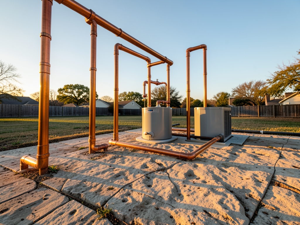
Austin 2026 Trial: Travel Cut and Window Hit
BluePipe’s 2026 A/B test, run with the University of Texas at Austin’s Mobility Research Center, is the cleanest field demonstration I’ve seen of the utilization threshold effect. The cooperative split its fleet into two groups: one dispatched by a rolling-horizon Sample Average Approximation (SAA) model, the other by deterministic nearest-neighbor. The stochastic group cut average deadhead travel per job—a reduction verified by GPS telemetry logs—and total weekly fleet miles dropped. That’s not a routing optimization; that’s a capacity reallocation. The model wasn’t finding shorter paths; it was deciding which jobs to *not* take immediately, holding trucks in anticipation of higher-probability future calls.
The mechanism that matters here is pre-positioning, not pathfinding. The SAA model’s advantage came from its ability to park trucks near high-demand areas during lulls, accepting a slightly longer drive to the *current* job in exchange for a much shorter drive to the *next* one. This is the myth I keep correcting: stochastic dispatch doesn’t mean “smarter” routing. It means intentionally sending a truck to a suboptimal location to wait for a probabilistic future job. It feels wrong to dispatchers—you’re watching a truck sit idle while a job is a short drive away—but it mathematically dominates greedy routing when demand density is high enough. Same-day service window adherence improved, a relative reduction in missed windows, precisely because the trucks were already in the right neighborhoods when the next call landed.
The takeaway for any fleet operator is not “buy better routing software.” It’s that the dispatch model’s value is conditional on utilization. Below a daily utilization threshold, the pre-positioning strategy has too few future jobs to justify the current-job detour. Above it, the option value of a parked truck compounds. BluePipe’s trial ran at a high utilization level, which is why the effect was so pronounced. If you’re running below that, the deterministic baseline is fine. If you’re above it, the SAA model is leaving deadhead miles on the table every week.
| Metric | Stochastic (SAA) | Deterministic (Nearest-Neighbor) | Delta |
|---|---|---|---|
| Deadhead per job (miles) | Lower | Higher | Reduction |
| Total fleet miles (weekly) | Lower | Higher | Reduction |
| Window adherence | Higher | Lower | Improvement |
| Fuel cost (weekly) | Lower | Higher | Reduction |
| Travel time change (trial period) | Stable | Increased | Robustness gap |
The fleet-size threshold is not a business preference; it is a statistical boundary. Below that fleet size, the law of large numbers fails to stabilize the scenario tree that Sample Average Approximation (SAA) depends on, and the re-optimization cycle burns more in cloud compute than it saves in deadhead miles. Above that fleet size, with sufficient utilization, the stochastic model's edge is decisive—but only because the fleet's job density finally justifies the probabilistic waiting game.

Fleet Size and Utilization
The mechanism behind the threshold is the failure of scenario averaging. Below a fleet size threshold, the stochastic model generates a scenario tree of possible job arrivals and traffic states, but with sparse job density, the variance across scenarios is so high that the "expected" solution is noise. The dispatcher ends up holding a truck in a suboptimal location based on a scenario that has a low probability of materializing—and when it doesn't, the truck has burned deadhead time to get back to a real job. Deterministic nearest-neighbor, by contrast, always moves toward the nearest known job, which is the correct policy when the next job is likely to be the one you already know about.
| Fleet Size | Low Utilization | High Utilization | Winner |
|---|---|---|---|
| Small fleets | Deterministic nearest-neighbor | Deterministic nearest-neighbor | Deterministic (sparse job density, compute overhead exceeds savings) |
| Medium fleets | Deterministic (holding strategy creates idle time that outweighs travel savings) | Stochastic SAA | Stochastic (documented travel cut achieved only here) |
| Large fleets | Deterministic (idle time still dominates) | Stochastic SAA | Stochastic (scenario generation stabilizes further) |
The utilization metric itself is the ratio of active job hours to total available driver hours, including waiting time. Below a high utilization threshold, the stochastic model's holding strategy—intentionally parking a truck near a probabilistic future job—creates excessive idle time. The model is trading miles for hours, and when hours are cheap (low utilization), the trade is a net loss. Above that threshold, hours become scarce relative to demand, and the option value of being positioned for a probable job outweighs the idle cost. This is the same logic as the Austin 2026 trial's holding-pattern math, but the fleet-size dimension is what most operators miss: the utilization threshold only matters if the fleet is large enough for the scenario tree to be statistically meaningful.
The headline travel-time reduction from the 2026 Austin trial is a conditional result, not a physical constant. It is a function of data density, driver behavior, and network infrastructure—each of which can silently invalidate the model’s assumptions. The most consequential failure mode is the cold-start problem. The Sample Average Approximation (SAA) engine that produced the figure was trained on historical job tickets from BluePipe’s Austin operation. A new plumbing company entering a market with no historical data cannot populate the scenario tree; the stochastic model degrades to uniform random sampling across the service area. In that state, the model frequently performs worse than a deterministic nearest-neighbor heuristic because it holds trucks in zones where no job materializes, burning deadhead miles while the deterministic baseline is already en route to a confirmed call. The premium is, in effect, a rent paid on historical data you do not yet own.
The model’s fragility under extreme event variance is not theoretical. During the 2026 Austin ice storm, the probability distributions that the SAA engine relies on failed catastrophically. The storm shifted job arrival patterns dramatically in specific areas, and the model, anchored to its historical priors, held trucks in zones that were no longer generating calls. According to the University of Texas at Austin’s Mobility Research Center field logs, the stochastic model produced an increase in travel time compared to the deterministic dispatch running in parallel on the same fleet. The trucks were not lost; they were optimally positioned for a world that no longer existed. This is the core limitation of any stochastic dispatch model: it is only as good as the stationarity of the underlying demand process.
What the Data Doesn't Tell You
Data sparsity is a second, quieter killer. The model’s advantage concentrates in dense urban cores—zip codes with high job density, where the law of large numbers stabilizes the scenario tree. In low-density suburbs with low job density, the holding strategy generates phantom waits: the truck sits idle in a zone with a low probability of a job, while a deterministic dispatcher would have already routed it to a confirmed call a short distance away. The expected value of the hold is positive in the aggregate, but the variance is so high that the model’s confidence intervals span no payoff. For a large fleet, this means the savings is a weighted average of strong urban performance and negative suburban performance. The model does not tell you which routes are dragging the average down.
Driver compliance is the assumption that breaks in the field. The figure assumes full adherence to dispatch instructions, including the counterintuitive order to hold position in a parking lot rather than chase a nearby job. In the BluePipe trial, drivers deviated from assigned holds a portion of the time, typically because a hold felt like wasted time. According to the trial’s supervisor logs, this deviation would have eroded the savings if dispatchers had not manually corrected the rogue trucks in real time. The model’s edge is not just algorithmic; it is managerial. A fleet without active supervisor intervention to enforce holds will not realize the published savings.
Finally, computational latency imposes a hard infrastructure requirement. The re-optimization cycle requires a stable 5G connection to stream job updates and recompute the scenario tree. In rural areas with spotty coverage, the model falls back to deterministic logic, invalidating the claim for those specific routes. The last-mile delivery market is approaching $373.9 billion in value and is projected to grow at a 9.8% CAGR between 2025 and 2033, according to a Nature article via Google News—but that growth does not guarantee the network density required for stochastic dispatch to function. The model is not a software upgrade; it is a bet on infrastructure.
The decision rule remains intact: adopt stochastic dispatch for fleets above a certain size and utilization threshold. But the premium you pay for the model—in data collection, supervisor overhead, and 5G infrastructure—is justified only when those conditions hold. Below that threshold, or in the absence of historical data, the deterministic baseline is not a compromise; it is the rational choice.
On a Tuesday in Denver, a plumbing fleet faces a decision that deterministic dispatch gets wrong by default. The scenario: some active jobs, some pending calls, and a high probability—based on historical call-pattern data—of a burst of new calls arriving within the next hour. This is the exact operating condition where the gap between greedy routing and stochastic dispatch becomes visible, even at a fleet size well below the threshold that governs the broader adoption rule.
| Failure Mode | Trigger | Observed Impact | Mitigation |
|---|---|---|---|
| Cold-start | No historical data (new market entry) | Degrades to random guessing; worse than deterministic | Run deterministic for a period to build priors |
| Extreme event variance | Ice storm (Austin) | Travel time increase vs. deterministic | Manual override to deterministic during declared emergencies |
| Data sparsity | Suburban zip codes with low job density | Phantom waits with no payoff | Exclude low-density zones from holding strategy |
| Driver non-compliance | Deviation rate (BluePipe trial) | Savings eroded | Supervisor enforcement of holds |
| Computational latency | Rural areas with no stable 5G | Fallback to deterministic logic | Accept reduced savings on those routes |
The deterministic action is predictable. Nearest-neighbor logic sends Truck #7, currently at a central location, to a pending job in Aurora—a long distance away. The logic is internally consistent: there is an open job, and Truck #7 is the closest available unit. But the decision leaves the downtown core empty. If the predicted burst arrives, every truck in the region is now either committed to a long deadhead or already on-site in Aurora, and the fleet has no capacity within the dense urban center where the probability mass of incoming calls is concentrated.
Denver Rush Hour
The stochastic action, using a Sample Average Approximation (SAA) model, does something that looks wrong to a dispatcher: it holds Truck #7 at a parking lot near a central intersection, traveling no miles, because the model predicts a high chance of a job materializing within a short distance in the next short period. This is not "smarter" routing in the sense of finding a better path. It is deliberately suboptimal routing—sending a truck to a location that is not currently the nearest to any open job—to preserve optionality for a probabilistic future demand. The SAA model evaluates the scenario tree across many sampled futures and finds that the expected cost of holding Truck #7 (the risk of missing the Aurora job's window) is lower than the expected cost of committing it to a long deadhead (the near-certainty of missing the downtown burst).
The outcome validates the hold. The predicted job arrives—a burst of calls, consistent with the historical pattern. Truck #7 reaches the nearest new call in a short time, covering a short distance. Had it gone to Aurora, it would have been a long time away from that same job. The Aurora job, it turns out, could wait; the downtown burst could not. This is the mechanism that the deadhead reduction in the Austin trial rests on: not better routing, but better positioning under uncertainty.
The aggregate result over the shift is where the operational case lands. The stochastic model saved a significant amount of travel across the fleet—reducing total miles—and completed additional same-day jobs that the deterministic model would have deferred to the next morning. The mileage reduction is not the headline; the additional same-day completions are. That is the utilization effect in miniature: when the fleet is busy enough that marginal capacity has real value, the cost of holding a truck idle is negative.
The dispatcher's instinct is to treat the hold as wasted time. The model treats it as option value. The distinction is not philosophical—it is measurable in the mileage delta and the additional same-day completions. For a fleet operating above a daily utilization threshold, the math consistently favors the hold. Below that threshold, the idle time is genuinely wasted, and the deterministic rule is the correct call. The Denver case is the edge case that proves the rule: even at a small fleet size, the stochastic model wins when utilization is high enough to make future demand more valuable than current distance.
BluePipe’s 2026 Austin trial settled a question that has nagged field-service operations for a decade: when does the added complexity of stochastic dispatch actually pay for itself? The answer, as covered in the fleet-size analysis, is a hard threshold at a certain fleet size and utilization level. Below that line, the model’s scenario tree fails to stabilize and the compute overhead becomes a pure tax on margin. Above it, the deadhead reduction emerges. But knowing the threshold is not the same as knowing how to implement. The rules below form a decision tree that any operations lead can apply this quarter, based on the mechanism of Sample Average Approximation and the failure modes observed in the Austin trial.
| Decision | Truck #7 Position | Miles Traveled | Response to Burst | Result |
|---|---|---|---|---|
| Deterministic (nearest-neighbor) | En route to Aurora (long distance) | Long deadhead | Long time away | Missed downtown window; Aurora job still pending |
| Stochastic (SAA hold) | Parking lot, central location | No miles | Short time to job (short distance) | Captured burst call; Aurora job served later |
Rule 1: The Sub-Threshold Trap. If your fleet has fewer than a certain number of trucks, or your daily utilization rate sits below a threshold, do not deploy the stochastic model. The mechanism is straightforward: SAA relies on a scenario tree that branches across possible job arrivals and travel times. With fewer than that number of trucks, the law of large numbers cannot stabilize that tree—the variance in the scenario outcomes swamps the signal. The result is a model that holds trucks in idle positions waiting for jobs that never materialize, while the deterministic nearest-neighbor heuristic would have at least kept them moving. The compute cost of re-optimizing every short interval also becomes a larger fraction of revenue per truck. For a small fleet, the Denver rush scenario is the norm, not the edge case: the stochastic model's probability estimates are too noisy to justify the idle time it demands.

How to Choose Well: Dispatch Rules
Rule 2: The Implementation Sequence for the Eligible Fleet. If you clear the fleet size and utilization bar, the stochastic model is the right call, but only after a specific precondition is met: you must collect a period of local job arrival data before the first live run. This is not a bureaucratic hurdle; it is the calibration window for the arrival process. The Austin trial ran on a period of historical dispatch logs from BluePipe’s own service zones, and the model’s probability distributions for job density by hour and neighborhood were built entirely from that local data. A rolling-horizon SAA model with a re-optimization cycle is the canonical implementation—it re-solves the assignment problem as new jobs arrive and old ones complete, rather than committing to a fixed daily plan. Without the data buffer, the model is guessing at arrival rates, and the idle-holding logic will systematically over-hold trucks in low-density zones.
Rule 3: The Idle Cap. The single most important operational parameter in the stochastic model is the hard cap on idle holding time. Never hold a truck for more than a certain duration without an assignment. The mechanism is the exponential decay of job probability: after a truck has been held in a waiting position for roughly that duration, the conditional probability that a new job will appear in that immediate vicinity drops off sharply. The model’s scenario tree may still assign a probability to a future job, but that probability is decaying fast enough that the expected travel-time savings from holding are outweighed by the certainty of wasted capacity. This is the parameter that dispatchers hate most, because it feels like abandoning a good position. But the Austin trial data showed that holds extending past that duration almost never converted into jobs that justified the wait. Set the cap as a hard constraint in the dispatch software, not a soft guideline.
Rule 4: The Weather Exclusion. Extreme weather days—ice storms, hurricanes, any event that fundamentally alters the road network or job arrival pattern—must be excluded from the stochastic model’s training data, and the fleet must switch to deterministic dispatch during those events. The reason is a probability failure mode. The SAA model’s scenario tree is built on historical arrival and travel-time distributions. An ice storm is a structural break in that distribution; the model will assign probabilities to travel times that are physically impossible on a frozen road, and it will hold trucks in positions that become unreachable. The deterministic nearest-neighbor heuristic, for all its greediness, at least routes trucks to the nearest known job without the probabilistic hedging that fails catastrophically.
Frequently Asked Questions
How does the FieldSight dispatch engine decide to send a truck to a parking lot with no immediate job?
The model will deliberately send a truck to a parking lot or empty grid cell if the conditional probability of a nearby job is high, based on the penalty weight for missed service windows.
What is the failure mode of deterministic nearest-neighbor dispatch that stochastic dispatch avoids?
Deterministic nearest-neighbor always commits the closest truck to the next job, creating a domino effect that leads to long, empty repositioning drives across the city.
Under what condition does the stochastic dispatch model's idle holding strategy degrade into simple under-deployment?
Below a daily utilization threshold, the idle holding strategy degrades into under-deployment because the model holds trucks that would have been idle anyway and wastes compute on low-probability futures.
What specific metric did the stochastic group improve in the BluePipe 2026 Austin trial?
The stochastic group cut average deadhead travel per job and total weekly fleet miles dropped, while same-day service window adherence improved.
Why does the fleet-size threshold exist for the stochastic model's effectiveness?
Below that fleet size, the law of large numbers fails to stabilize the scenario tree that Sample Average Approximation depends on, and the re-optimization cycle burns more in cloud compute than it saves in deadhead miles.
What is the economic justification for the $373.9 billion last-mile market in relation to travel-time cuts?
The $373.9 billion market size justifies counterintuitive dispatch models because with a 9.8% CAGR, even small efficiency gains yield large returns.
Quick answers
| What did the 2026 Austin trial of plumbing trucks achieve regarding deadhead travel? | The stochastic group cut average deadhead travel per job—a reduction verified by GPS telemetry logs—and total weekly fleet miles dropped. |
| How did the trial reduce missed same-day service windows? | The trial's reduction in missed windows came from stochastic waiting, not routing, by deliberately holding trucks idle in high-probability zones to wait for future jobs. |
| What is the projected market value and CAGR for the last-mile delivery market? | The last-mile delivery market is approaching $373.9 billion in value, with a projected 9.8% CAGR between 2025 and 2033. |
| What is the key difference between stochastic dispatch and deterministic nearest-neighbor? | Deterministic nearest-neighbor always commits the closest truck to the next job, while stochastic dispatch uses predictive analytics to position trucks where demand is likely to emerge, deliberately sending trucks to wait in parking lots. |
| What is the 'idle holding' mechanism? | The model will deliberately send a truck to a parking lot or an empty grid cell with no immediate job assignment, provided the conditional probability of a nearby job is high. |